Recently I was looking for useful graphs on recent parallel computing hardware for reuse in a presentation, but struggled to find any. While I know that colleagues have such graphs and data in use in their presentations, I couldn't find a convenient source on the net. So I ended up collecting all the data (again) and decided to make the outcome of my efforts available here.
Wikipedia already provides extensive lists on AMD graphics processing units as well as NVIDIA graphics processing units. For CPUs I restricted my comparison to the family of INTEL Xeon microprocessors supplemented by INTEL's export compliance metrics for Xeon processors for simplicity, as the main trend would also hold true for AMD processors.
My comparison considers high-end hardware available by the end of the respective calendar year. All data for 2016 are preliminary. Multi-GPU boards are ignored because they only represent a small share of the market. Similarly, I only consider CPUs for dual socket machines, since this is also the baseline used by INTEL for comparisons with their MIC platform (aka. Xeon Phi). Numbers for the Xeon Phi were taken directly from an INTEL PDF on the Xeon Phi.
>> GitHub repository with raw data, Gnuplot scripts and figures <<
Power Consumption
Let us start with a look at power consumption. The main reason for the introduction of parallel architectures were power constraints, as the electric power consumed by CPUs and GPUs (and thus the heat generated) increases in good approximation with the cubic power of clock frequency. You might want to have a look at my 40 Years of Microprocessor Trend Data blog post for additional data. For practical reasons of cooling, all mainstream computing hardware today is limited to about 250 to 300 Watts:
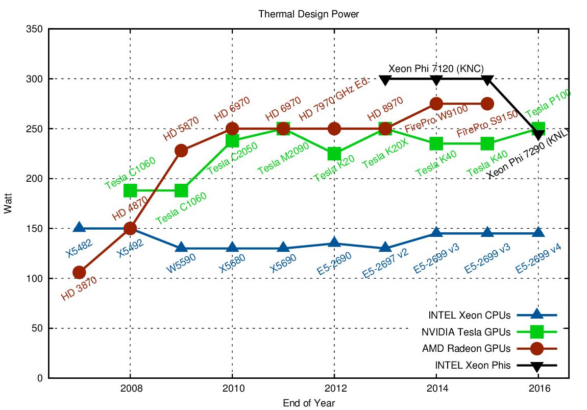
Comparison of the thermal design power of high-end hardware over time. Lower is preferable.
CPUs generally are designed for only half the thermal design power (TDP) when compared to a single GPU, hence a fair comparison in terms of power and performance should be based on a dual socket system versus a single GPU. It should also be noted that the peak performance consumption can sometimes exceed the TDP by a significant margin, as a number of reviews such as this comparison of a Radeon HD 7970, a Radeon HD7950, and a GeForce GTX 680 suggest. Dynamic clock frequency techniques such as those used for CPUs have recently been adopted by GPU vendors and may further drive up the short-term power consumption. Consequently, the TDP plateau will remain at about this level, while power supplies are likely to increase their peak power output for some time in order to handle higher short-term power consumption. The Xeon Phis are no different than GPUs in terms of power consumption and should also be compared against a dual-socket CPU system.
Raw Compute Performance
Accelerators and co-processors are - nomen est omen - great for providing high performance in terms of floating point operations (FLOP) per second. Consequently, it is no surprise that the effectiveness of GPUs for general purpose computations is often reduced to their pure FLOP rates, even though this may be the totally wrong metric as will be discussed later.
Since NVIDIA provides dedicated product lines focusing on either single or double precision arithmetic, we consider the two separately. Even though the hardware is very similar or even identical among these two product lines, the pricing is substantially different. ECC memory, large GPU RAM, and high performance for double precision arithmetic comes at a premium. AMD started to stronger differentiate their consumer and professional product lines with their Graphics Core Next architecture as well, but for the time being it is not necessary to differentiate the two.
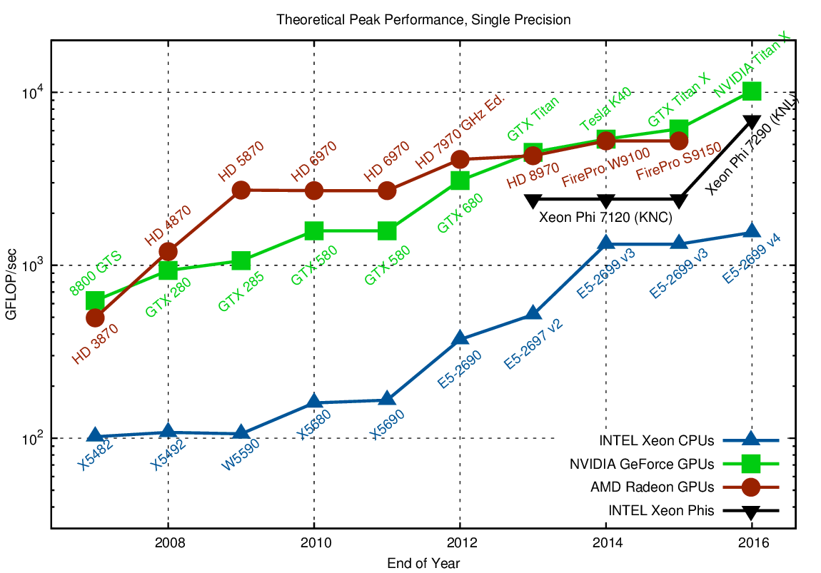
Comparison of theoretical peak GFLOP/sec in single precision. CPU data is for a single socket. Higher is better.
The comparison of theoretical peak performances for single precision arithmetic shows a five- to fifteen-fold margin when comparing high-end CPUs with high-end GPUs. This margin largest around 2009, when general purpose computing on GPUs (GPGPU) took off. The introduction of Xeon CPUs based on the Sandy Bridge architecture (with support for AVX) in 2012 and the dual-issue floating point units introduced with Haswell in 2014 reduced the gap between CPUs and GPUs. The recent introduction of NVIDIAs Pascal architecture widened the gap to a factor of about three when comparing a single GPU with a dual-socket system. What is not entirely reflected in the chart is the fact that the practical peak on the GPU is often further away from the theoretical peak than for the CPU; but even when taking this into account, the GPU is slightly faster. The Xeon Phi product line fills the gap between CPUs and GPUs when it comes to single precision arithmetic. For double precision arithmetic, the Xeon Phi is very close to the performance of GPUs:
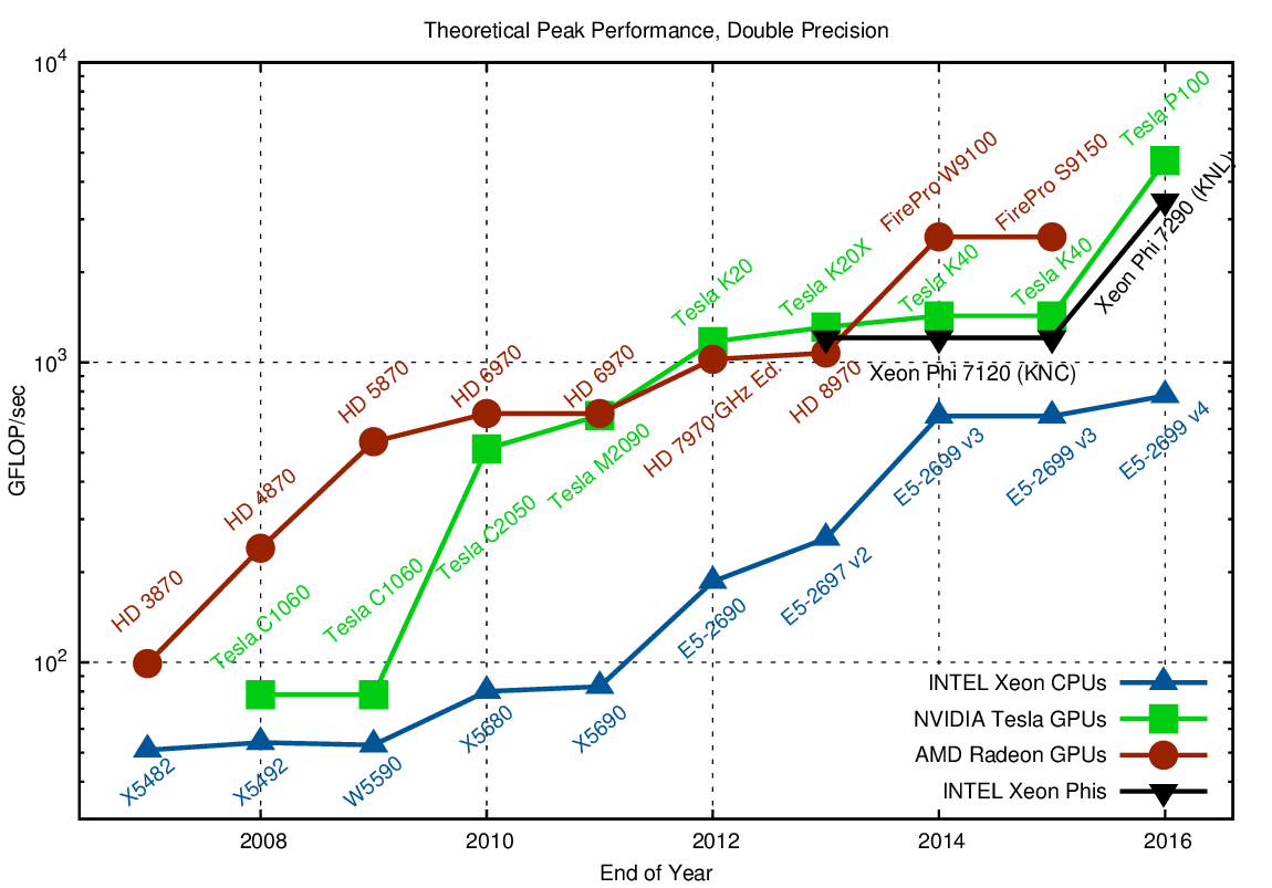
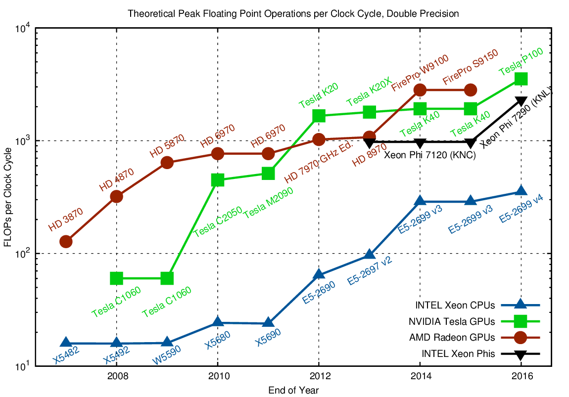
Comparison of theoretical peak GFLOP/sec in double precision. CPU data is for a single socket. Higher is better.
The difference in performance between single precision and double precision arithmetic of current GPUs can be up to a factor of 32. This is different from CPUs, where the factor is two. Consequently, CPUs almost closed to gap with the Haswell architecture in 2014. What is also interesting to see is that GPUs were virtually unable to deal with double precision arithmetic before 2008, so it took until 2010 until one could see a significant theoretical gain over the CPU. Also, AMD had a good advantage over NVIDIA at that time, even though it was NVIDIA who pushed general purpose computations back then. Today, a dual socket CPU-based system is within about a factor of three with respect to GPUs and Xeon Phis when it comes to theoretical double precision peak performance. All three massively parallel architectures (AMD GPUs, NVIDIA GPUs, INTEL Xeon Phis) provide virtually the same peak performance, so a preference of one architecture over another should be based on development effort, maintainability, and portability aspects rather than minor differences in peak performance.
Raw Compute Performance Per Watt
Since power is the limiting factor in computing today, let us have a look at FLOPs per Watt in both single and double precision arithmetic:
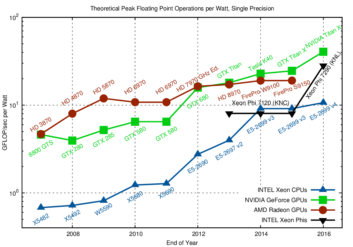
Comparison of GFLOP/sec per Watt for single precision arithmetic. Higher is better.
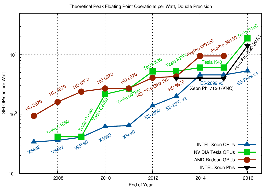
Comparison of GFLOP/sec per Watt for double precision arithmetic. Higher is better.
For a massively parallel algorithm with fine-grained parallelism such as dense matrix-matrix multiplications, GPUs and Xeon Phis provide about a three- to four-fold advantage when compared to CPUs. The gap in power efficiency in 2016 is smaller than in the 2007-2010 time frame, indicating a slow convergence of architectures. In fact, INTEL CPUs introduced wider vector units (up to 512 bits with KNL and Skylake), making their arithmetic units more GPU-like. Hence, the efficiency gap is unlikely to increase in the future.
Number of Cores
The question of how to define and compare 'cores' in CPUs and GPUs is tricky. In the first edition of this blog post, I compared physical CPU cores with GPU processing units. However, processing units in GPUs are not truly independent, but rather clever extensions of technology formerly part of vector computers. Thus, rather than comparing thousands of scalar GPU 'cores', which are part of big SIMT/SIMD engines, with CPU SIMD cores, I compare streaming multiprocessors (NVIDIA) and compute units (AMD) with CPU cores:
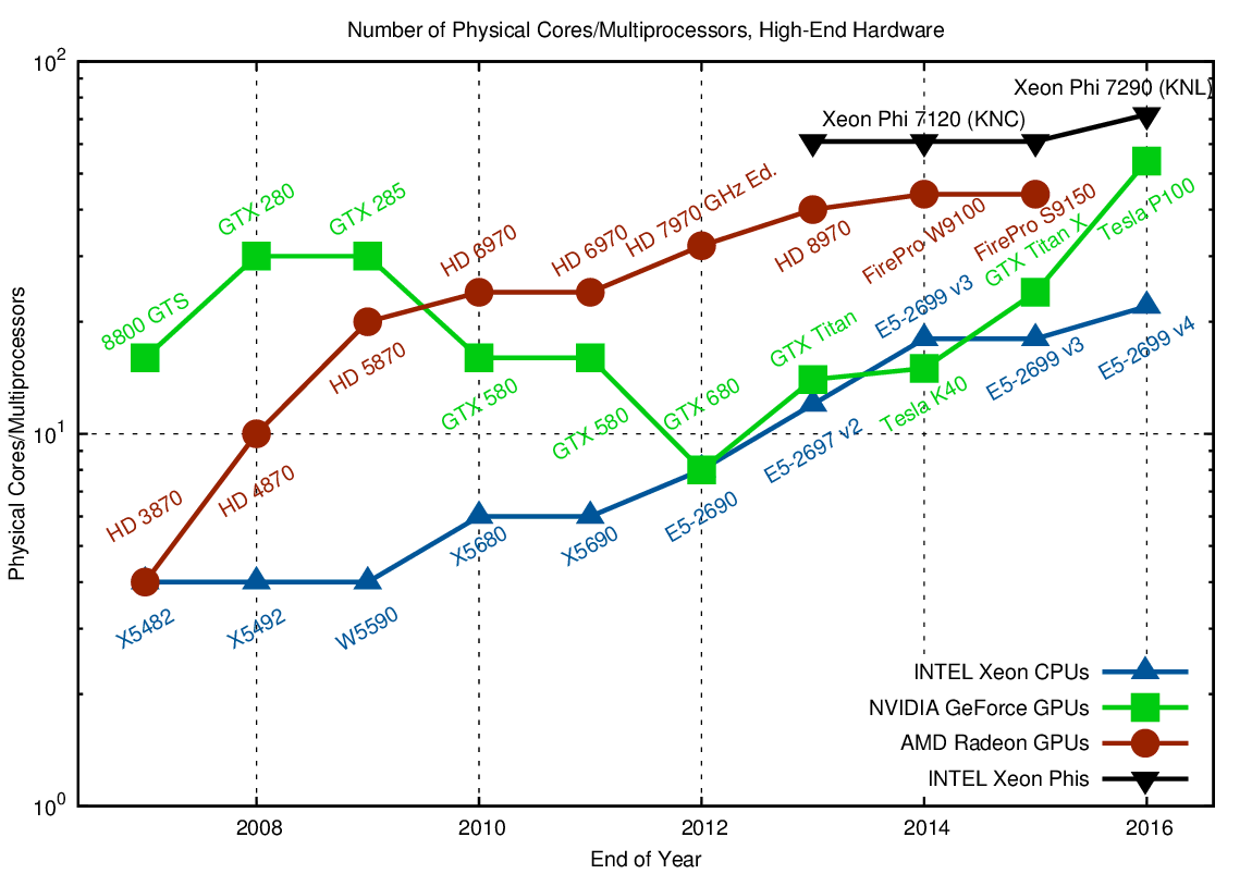
Comparison of cores and multiprocessors for high-end hardware using single precision arithmetic.
NVIDIAs strategy with Fermi and Kepler between 2010 and 2014 is fairly remarkable: Rather than increasing the number of streaming multiprocessors, the number went down. Thus, more processing units were squeezed into a single streaming multiprocessor. This resulted in better performance of a single streaming multiprocessor, which was useful for a algorithms that could not be easily scaled to multiple streaming multiprocessors.
Per-Core Performance
With the above definition of a 'core', let us have a look at per-core performance:
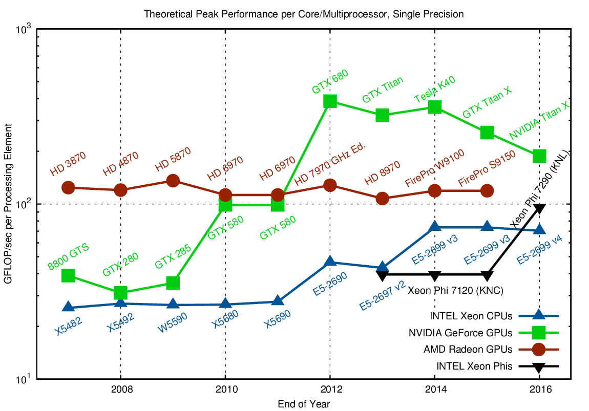
Comparison of GFLOP/sec contributed by each processing element or core when using single precision arithmetic.
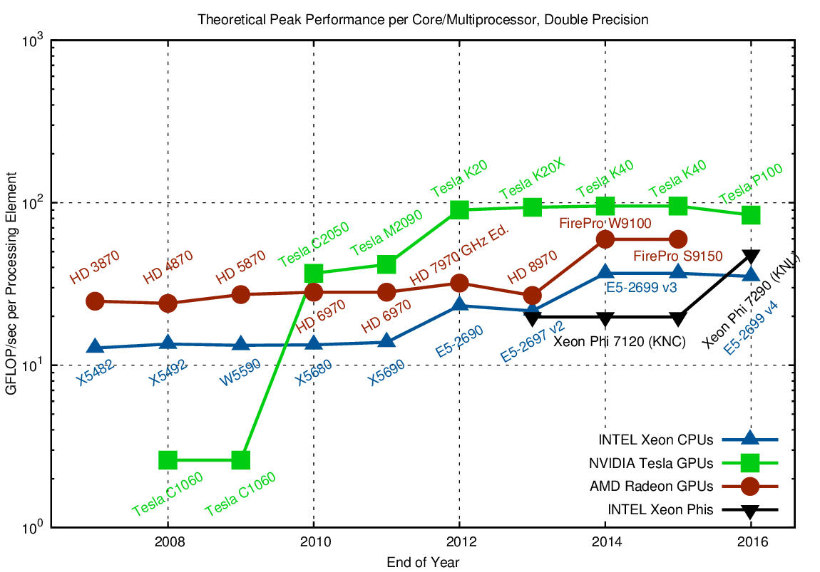
Comparison of GFLOP/sec contributed by each processing element or core using double precision arithmetic.
The plots for single and double precision arithmetic show interesting architectural decisions: While the per-core performance of AMD GPUs is almost constant over the years, NVIDIAs Fermi architecture (2010-2011) and Kepler architecture (2012-2015) show a significant increase in per-core performance over their previous generations. Also, one can clearly see how Kepler was optimized for high FLOP rates within a single streaming multiprocessor. Interestingly, the Maxwell and Pascal architectures reduce per-core performance and instead focus on a higher number of streaming multiprocessors.
Changes in the per-core performance of INTEL CPUs can be pinpointed directly: Additional vector instructions via AVX in Sandy-Bridge in 2012 and a second floating point unit with Haswell in 2014 each increase the per-core performance by a factor of two. However, AVX is not a general purpose solution for sequential performance. In other words: Sequential general-purpose performance stagnates and regular, vector-friendly data layout is the key to good performance.
The suggested good single-core performance of the Xeon Phi in the charts above might come by surprise. However, keep in mind that transistors have been spent on arithmetic units rather than caches and the like. Thus, based on the two charts one must not conclude that the Xeon Phi provides high sequential performance just like conventional CPUs. Nevertheless, it is well reflected in the charts above that the Xeon Phi is essentially a collection of CPU cores rather than a GPU-like architecture.
Memory Bandwidth
In order to use all arithmetic units efficiently, the respective data must be available in registers. Unless the data are already available in registers or cache, they need to be loaded from global memory and eventually be written back at some later point. These loads and stores are a bottleneck for many operations, which CPUs to some extent mitigate by large caches. However, we will ignore any influences of caches and only compare memory bandwidth to global memory (see E. Saule et al. for a reference to the ring-bus bandwidth on the Xeon Phi):
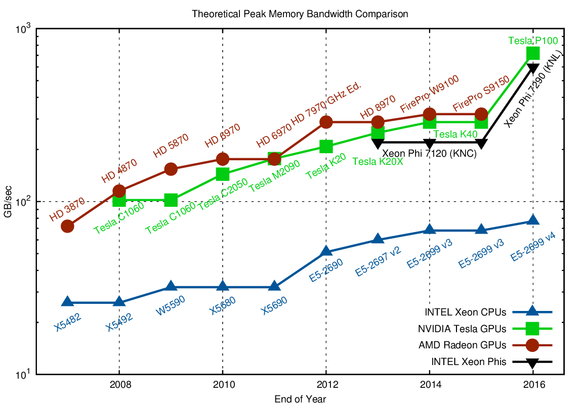
Comparison of theoretical peak memory bandwidth. Higher is better. Note that the MIC uses an internal 220 GB/sec ring-bus, which is the limiting factor over the ~320 GB/sec provided by the memory controllers. The theoretical peak memory bandwidth for the Xeon Phi 7290 was extrapolated from the STREAM benchmark bandwidth of approx. 490 GB/sec.
In contrast to raw performance, the advantage of GPUs and Xeon Phi over a single CPU socket in terms of peak memory performance has increased from about three-fold in 2007 to ten-fold in 2016. The introduction of high bandwidth memory (MCDRAM for Xeon Phi, stacked memory for NVIDIA) in 2016 is a major selling point of GPUs and Xeon Phis over CPUs. Time will tell whether high bandwidth memory will become available for Xeon CPUs; after all, I claim that high bandwidth memory is the only significant difference between the Xeon and the Xeon Phi product lines.
There is also lot to be said and compared about caches and latencies, yet this is well beyond the scope of this blog post. What should be noted, however, is a comparison with PCI-Express memory transfer rates: A PCI-Express v2.0 slot with 16 lanes achieves 8 GB/sec, and up to 15.75 GB/sec for PCI-Express v3.0. This is at best comparable to a single DRAM-channel.
Floating Point Operations per Byte
Whenever data needs to be loaded from global memory to feed the arithmetic units, a significant imbalance shows up, commonly referred to as the memory wall. For example, if you want to add up the numbers in two buffers of length N and store the result in a third buffer, all using double precision, you need to load 2N*sizeof(double) = 16N bytes from memory, and write N*sizeof(double) = 8N bytes back, using a total of N arithmetic operations. Ignoring address manipulations for loads and stores, only 1/24 FLOPs per transferred byte are required. Similarly, even operations such as dense and sparse matrix-vector operations are usually well below one FLOP per byte. Hence, higher FLOP-per-byte ratios indicate that only few algorithms can fully saturate the compute units. Conversely, to make all algorithms compute-bound, one would need infinite memory bandwidth (i.e. a FLOP-per-byte ratio of zero). With this in mind, let us have a look at FLOP per byte ratios of high-end hardware:
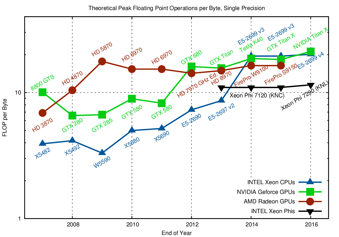
Comparison of required floating point operations per byte when using single precision arithmetic in order to transition between compute-limited and memory-bandwidth-limited regimes.
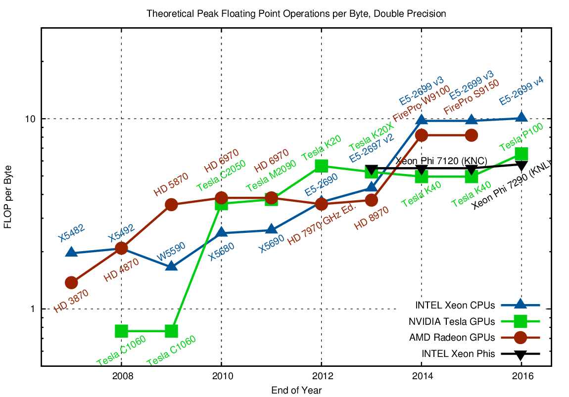
Comparison of required floating point operations per byte when using double precision arithmetic in order to transition between compute-limited and memory-bandwidth-limited regimes.
Both CPUs and GPUs offer very high FLOP-per-byte ratios. Somewhat counter-intuitive, CPUs today show the highest FLOP-per-byte ratios. This is mostly due to the relatively slow DDR3/DDR4 memory channels, while GPUs and Xeon Phis use GDDR5/GDDR5X or high bandwidth memory links. Regardless, the trend to higher FLOP-per-byte ratios is readily visible. Even high memory bandwidth could not reduce the ratio; every additional GB/sec of memory bandwidth results in at least the same increase in floating point capabilities.
Overall, the general guideline is (and will continue to be) that FLOPs on CPUs, GPUs and Xeon Phi are for free. Thus, the problem to tackle for future hardware generations is memory, not FLOPs. Another way to put it: Reaching Exascale is at least partially about solving the wrong problem.
Floating Point Operations per Clock Cycle
When talking about parallelism, one frequently talks about the number of cores. 22 CPU cores in a high-end Xeon CPU sound like a lot, but are few compared to the 3584 processing units (see discussion of 'cores' above) in a GPU. Let us have a look at the number of floating point operations within a single clock cycle, because this is another, less common metric for parallelism. In particular, details of cores, vector registers, lock-step execution, and the like are no longer important. To condense everything into a simple question: How big is the difference of using the full device (all floating point units busy) versus running a sequential, non-vectorized code after ignoring all cache and memory bandwidth and latency issues?
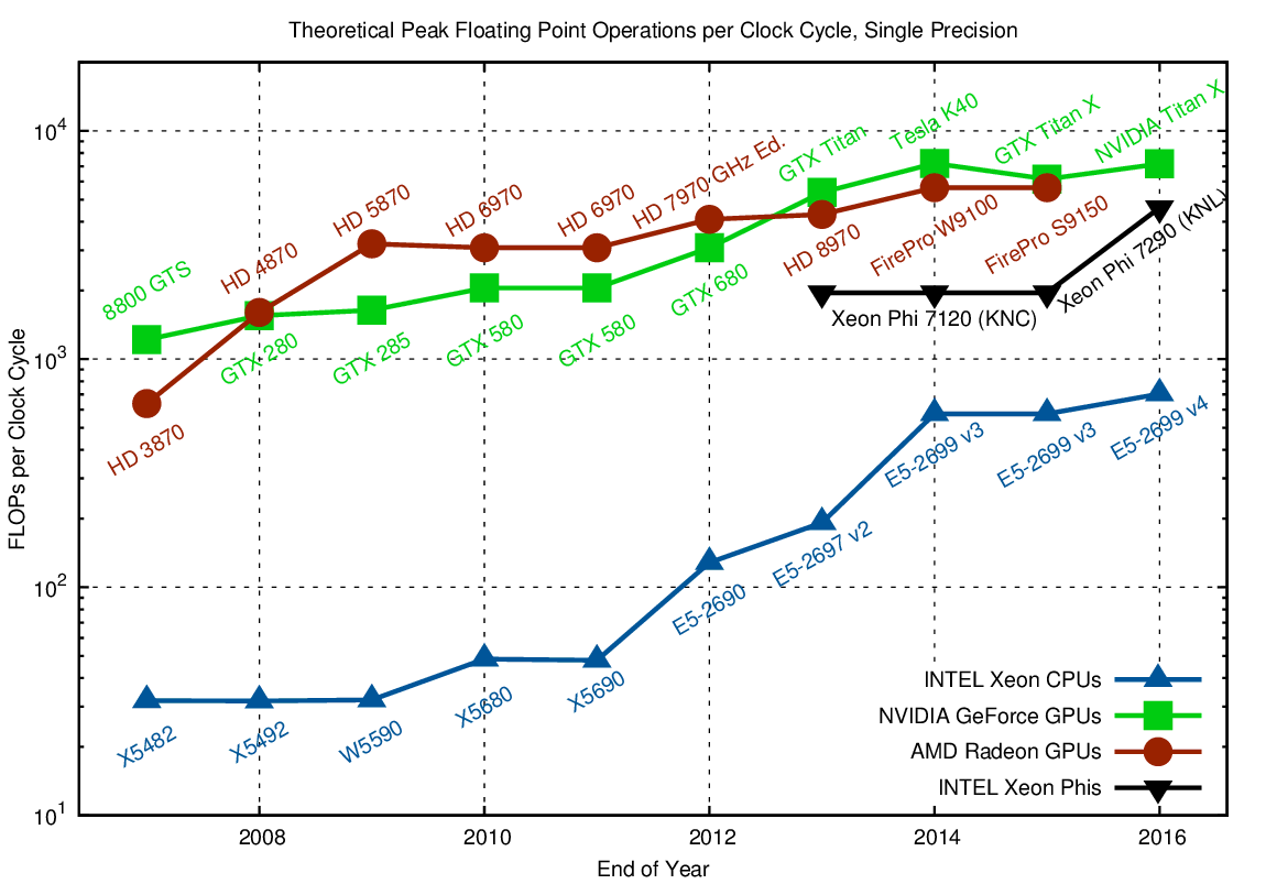
The number of FLOPs per clock cycle (unity for a purely sequential CPU) is in the tens for CPUs and in the hundreds for GPUs and Xeon Phi. Only parallelization and vectorization can leverage the full potential.
The number of FLOPs per clock cycle (unity for a purely sequential CPU) is in the tens for CPUs and in the hundreds for GPUs and Xeon Phi. Only parallelization and vectorization can leverage the full potential.
The charts for both single and double precision arithmetic show that CPUs in 2016 are already similar to GPUs in 2007-2008 in terms of FLOPs per clock cycle. The introduction of AVX512 in the upcoming Skylake Xeon CPUs will double the number of FLOPs per cycle again, further closing the gap between CPUs, GPUs, and Xeon Phis. Given this pending convergence of massively parallel architectures, there is little reason to worry about a particular architecture. If you use the right algorithms, you will be well prepared for any architecture 🙂
Summary
The comparison of main hardware characteristics did not show any unexpected results: GPUs and Xeon Phis are good for FLOP-intensive applications, but performance gains by much more than about an order of magnitude over a comparable CPU are certainly not backed up by hardware characteristics. It will be interesting to see how the FLOP per byte ratio will develop in the near future, as the raw processing count keeps increasing at a higher pace than the memory bandwidth. Also, I'm looking forward to a tighter integration of traditional CPU cores with GPU-like worker units, possibly sharing a coherent cache.
Raw Data
Check out my GitHub repository containing all raw data, all the Gnuplot scripts for the figures, and a Bash script for generating them all with a simple call. All content is available via a permissive license so that you can reuse the plots in reports, alter as needed, etc.:
>> GitHub repository with raw data, Gnuplot scripts and figures <<
Change Logs
Edit, June 24th, 2013: As Jed Brown noted, GFLOP/sec values for CPUs were missing a factor of two due to a single- vs. double-precision lapse. This is now corrected. Thanks, Jed!
Edit, June 13th, 2014: Updated graphs and text to consider INTEL CPUs available by the end of 2013.
Edit, March 25th, 2014: Updated graphs and text for hardware available by the end of 2014.
Edit, August 18th, 2016: Updated graphs and text for hardware available by mid 2016. CPU cores are now compared against GPU multiprocessors. Added plot of FLOPs/cycle. Thanks to Axel Hübl for his encouragement.
Dear Mr. Rupp,
thank you for this nice summary.
What I would be interested additionally is a graph like
GFlop/s/USD
taking into account the price of the supercomputer.
Can you say something about that?
Kind regards, Andreas Will
Hi Andreas,
I thought about adding such a price tag comparison, but finally decided not to include it here because for supercomputers the acquisition costs have lower emphasis over power consumption, cooling, etc.
Also, in many cases one better compares Memory Bandwidth per Dollar, bringing in costs for the network, etc.
We have some continued discussion about system costs here, I may discuss this (including total system power consumption) soon in another post (no promises, though...)
Best regards,
Karli
A very interesting comparison.
However, I do believe that we, as practitioners, should seek to better define what we mean by a core. The industry seems to have adopted two different, mutually incompatible, definitions of the word: one for CPUs (including the MIC) and another for GPUs.
Most people would classify the Intel Core i7 2600K chip in my desktop as having 4 cores and the NVIDIA GTX 580 GPU as having 512 cores. However, the cores in my CPU are linearly independent whereas those in my GPU are not. The CUDA equivalent of a CPU core is an streaming multi-processor; of which my GPU possesses 16 of.
Going in the other direction let us reconsider the CPU. While it does indeed have 4 cores it also features hyper-threading technology, bringing us up to 8 cores. Each of these cores has a 256-bit vector unit capable of processing eight single precision numbers at a time. Hence we can have 8*8 = 64 streams in flight at once. Further, if my algorithm does not require all of the 16 available vector registers I can begin to utilise software pipe-lining to further increase throughput (in certain scenarios, anyway). Hence, I may be able to have 128 streams in flight. Both of these numbers are an order of magnitude more than the number of cores.
The key observation is that to obtain peak FLOPs on a CPU is that you have to be vectorizing your code. By far the most practical means of accomplishing this is to process multiple streams in parallel. Hence, a CPU is really not all that different from a GPU. Reworking the presented graphs to be in terms of data streams rather than cores would show the CPU and GPU to be a lot closer than many people think.
Regards, Freddie.
Pingback: PyViennaCL: GPU-accelerated Linear Algebra for Python | Karl Rupp
Pingback: Data Science with Python: Getting Started - The Hour News