While processor manufacturers repeatedly emphasize the importance of their latest innovations such as vector extensions (AVX, AVX2, etc.) of the processing elements, proper placement of data in memory is at least equally important. At the same time, generic implementations of many different data structures allow one to (re)use the most appealing one quickly. However, the intuitively most appropriate data structure may not be the fastest.
Let us consider the transposition of a sparse matrix A. Such an operation shows up in algebraic multigrid methods for forming the restriction operator from the prolongation operator, or in graph algorithms to obtain neighborhood information. A only has a small number of nonzero entries per row, but can have millions of rows and columns. Clearly, a dense storage of A in a single array is inappropriate, because almost all memory would be wasted for storing redundant zeros. Most practical implementations use a row- or column-oriented storage of A, where for each row (or column) the index and the value of each entry is stored. A simple way of transposing a sparse matrix is to reinterpret a row-oriented storage of A as column-oriented (or vice versa), but we will consider an explicit transposition of matrix A in row-oriented storage into a matrix B=AT with row-oriented storage. Any results obtained subsequently will hold true for the case of column-oriented storage as well.
Storage Schemes
Three storage schemes are compared in the following. The first two represents "off-the-shelf" approaches using the C++ STL and Boost. The third scheme is more C/Fortran-like, as it uses continguous memory buffers at the expense of a less convenient interface.
STL Vector of STL Maps
One way to account for the few nonzeros per row in A is to store each row of A as binary tree (std::map in the C++ STL). Since A usually has no empty rows or columns, there are no empty trees and hence no memory wasted. Thanks to operator overloading, we can thus quickly set up a matrix object which only stores the nonzeros of a matrix:
// set up A with 10 rows:
std::vector<std::map<int, double> > A(10);

// write some nonzeros to A:
A[0][4] = 42.0;
A[8][2] =  1.0;
...
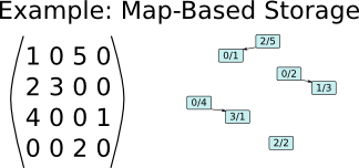
Example of storing a sparse matrix with 0-based indices using one binary tree (std::map or boost::flat_map) per row.
STL Vector of Boost Flat Maps
STL maps typically allocate new memory for each new element. Higher data locality and thus better cache reuse can be obtained by using an implementation where all elements of the map are stored in the same memory buffer. Unfortunately, the C++ STL does not provide such an implementation, but we can pick flat_map from Boost. Since the flat_map is interface-compatible with std::map, the code snippet above can be reused by merely changing the type:
// set up A with 10 rows:
std::vector<boost::container::flat_map<int, double> > A(10);

// write some nonzeros to A:
A[0][4] = 42.0;
A[8][2] =  1.0;
...
Similar to an STL vector, flat_map also allows to reserve memory for the expected number of entries to avoid memory reallocations. In the context of matrix transposition we can make use of knowing the expected average number of nonzeros per row. To allow for some headroom, a preallocation of twice the average number of nonzeros per row is used; empirical checks showed performance gains of 20 percent over this more pessimistic estimate.
CSR format
In the CSR format all column indices for each nonzero are stored row after row in a single buffer.
Similarly, all nonzero values are stored row after row in a single buffer. The entry points denoting the beginning of each row are stored in a third buffer, where the end of the i-th row is implicitly given by the start of the i+1-th row.
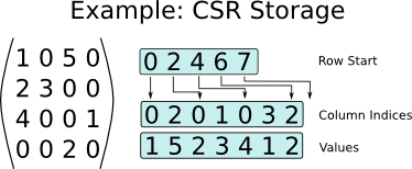
Example of storing a sparse matrix with 0-based indexing in the CSR format.
Managing data inserts into CSR is more challenging: In worst case, each new entry requires a copy of all existing entries in the matrix, entailing very high cost. Often one can work around these costs by first determining the sparsity pattern in a first stage and then writing the nonzero entries into a properly allocated sparse matrix in a second step. This is also how the sparse matrix transposition is implemented: First, the sparsity pattern of the result matrix is determined, then the entries are written. In contrast to the previous two data structures, column indices need to be accessed twice instead of only once. The drawback from a usability point of view is that the convenient bracket- or parenthesis-access C++ users are used to is almost always slow.
Benchmarks
In the following the execution times for transposing square sparse matrices using each of the three storage schemes described above are considered on a single core of an Intel Xeon E5-2670v3. The benchmark code is available on GitHub. Parallelization of sparse matrix transposition is very challenging and will be considered in a later blog post. The first matrix type carries 10 nonzeros per row, the second type has 100 nonzeros per row. The column indices of nonzeros in each row are selected randomly for simplicity. This is likely to entail higher cache miss rates than sparse matrices derived from graphs with ordering schemes such as Cuthill-McKee, yet the qualitative findings are the same.
Execution times for sparse matrices with different sizes and 10 nonzeros per row are as follows:
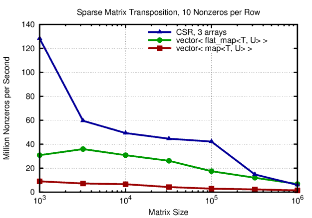
Performance of sparse matrix transposition with 10 nonzeros per row. Overall, the CSR storage scheme outperforms 'easier' storage schemes based on binary trees for the nonzeros in each row.
The performance differences are substantial: The CSR storage format benefits a lot from caches for low system sizes. For small matrices of size 1000x1000 the performance gain over flat_map and map is 4- and 12-fold, respectively. As matrix sizes increase, more cache misses are encountered, so the performance gap closes and ultimately CSR and flat_map reach the same performance of roughly 10 million nonzeros transposed per second. The performance of the implementation based on an STL map for each row is by a factor of four lower than the one based on flat_map.
The overall picture remains similar of 100 nonzeros per row are considered:
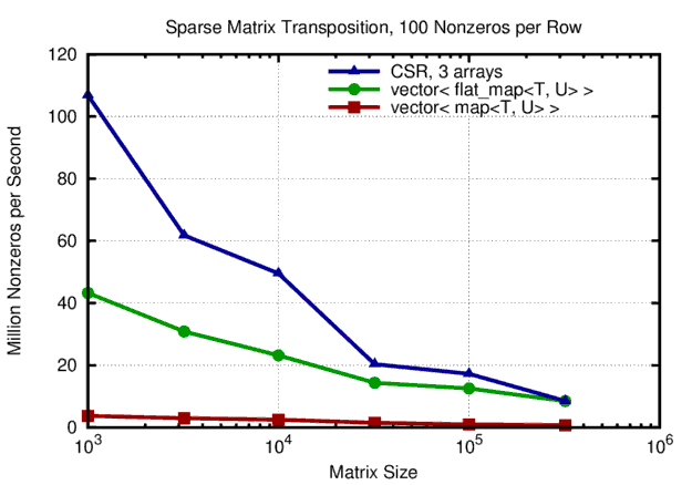
Performance of sparse matrix transposition with 100 nonzeros per row. Overall, the CSR storage scheme outperforms 'easier' storage schemes based on binary trees for the nonzeros in each row.
Again, CSR is about a factor of two faster than a vector of flat_map for smaller matrices. The two data storage schemes ultimately approaching the same performance for large matrices. Again, the implementation based on the STL map is almost uniformly by a factor of four slower than the implementation based on flat_map.
Finally, let us derive a simple performance model to evaluate possible further gains: At the very least, a sparse matrix transposition needs to load sizeof(int) + sizeof(double) bytes of data (column index and value) and write them to the result matrix. Thus, 24 bytes per nonzero entry in the initial sparse matrix need to be transferred. For a matrix with one million rows and ten nonzeros per row, 240 MB of data are moved. We thus achieved an effective bandwidth of 150 MB/sec with the observed execution time of 1.6 seconds, which is about a factor of 60 below the theoretical maximum of 10 GB/sec for a single memory channel. Considering that
- the CSR format requires a two-stage approach and thus column indices need to be loaded multiple times,
- additional memory transfers are required for initializing buffers and dealing with row indices,
- and that the unavoidable strided memory access suffers from significant performance hits with effective memory bandwidths on the order of only 1 GB/sec,
we can conclude that there is not too much (maybe 2x?) headroom for further improvement. One option is to consider parallelization, which is fairly tricky in this setting and will be covered in a later blog post. Another option is to reorder row and column indices to reduce the bandwidth of the matrix (and thus increase locality of data access). As with all sparse matrix operations, accurate predictions are difficult because everything depends on the nonzero pattern.
Conclusions
The benchmark results strongly suggest to favor flat arrays (CSR format) over flat_map from Boost over the STL map. This can be explained with only three words: Data locality matters. Since sparse matrix transposition is similar to several graph algorithms, our results suggest that tree-based datastructure should not be used carelessly if performance is of high important.
At the same time, not every piece of code should be optimized blindly: The implementations based on top of flat_map and map are significantly shorter and easier to maintain. Thus, if development time is more costly than execution time, they may still be the better choice.
This blog post is for calendar week 7 of my weekly blogging series for 2016.